rctopo
| author: | Stanislav Stoupin |
|---|---|
| email: | <sstoupin@gmail.com> |
x-ray rocking curve topography calculator
SYNOPSIS
rctopo [options] filename1 filename2 ... filenameN
DESCRIPTION
A program to process a sequence of images (topographs) collected at different angles on the rocking curve of a crystal to generate maps of the rocking curve parameters. Supported area detector file formats: HDF4 (.hdf), HDF5 (.h5), a variety of image formats (PNG, TIFF, JPG)
OPTIONS
For a brief summary run:
rctopo -h
| -h, --help: | |
|---|---|
show summary of options |
|
| -v, --version: | |
show program's version |
|
| -o FILENAME, --output FILENAME: | |
write calculated results to file (default to stdout); also, generates output prcurve.dat and trcurve.dat containing the rocking curve from the central pixel and the total rocking curve respectively |
|
| -w FILENAME, --output FILENAME: | |
write slice data to file (default: no action) |
|
| --hdf5 FILENAME: | |
save data and topographs to hdf5 file (default: no action) |
|
| -j, --tif: | |
save calculalted rocking curve topographs as tif files (default: no action) |
|
| -t CONST, --threshold CONST: | |
threshold CONST for data processing to define crystal boundaries (default T=1.05) |
|
| -b CONST, --background CONST: | |
user defined background CONST, e.g., dark current of the area detector (default: value is estimated from the rocking curve tails) |
|
| -r STRING, --range STRING: | |
xy-range for display and analysis (STRING='x1 x2 y1 y2', where x1,x2,y1,y2 are in units of [mm]) |
|
| -x CONST, --xslice CONST: | |
plot distributions (slices) at a fixed coordinate X = CONST |
|
| -y CONST, --yslice CONST: | |
plot distributions (slices) at a fixed coordinate Y = CONST |
|
| -f CONST, --factor CONST: | |
scale colormap range on FWHM and STDEV topographs by CONST*FWHM_av, where FWHM_av is the average FWHM |
|
| -m CONST, --magnify CONST: | |
scale colormap range for COM, Midpoint, Left Slope and Right Slope by factor CONST*FWHM_av, where FWHM_av is the average FWHM |
|
| -n STRING, --name STRING: | |
include sample name STRING in the figure title |
|
| -d CONST, --deglitch CONST: | |
deglitch data using median filtering, where CONST (an odd number, e.g., CONST=3) is the size of the filter window (default: no deglitching) |
|
| -g, --gaussian: | |
perform Gaussian curve fitting (smoothing of noisy data) |
|
| -s, --transpose: | |
transpose image array for plotting |
|
| -u uname, --units uname: | |
assign the original angular units (uname): deg, arcsec or urad (default: deg) |
|
| -p, --publish: | |
generate additional figures (requires user-defined figures.py script) |
|
| -c, --conduct: | |
process sequence of diffraction images collected in transmission mode |
|
| -i, --instrument: | |
read parameters from an instrument file ccd.py |
|
| -z CONST, --integrate CONST: | |
presentation of the intensity (reflectivity) map: CONST = 0 plot peak intensity normalized by the found maximum value (default) CONST = -1 plot integrated intensity normalized by the found maximum value otherwise (CONST !=0 and CONST !=-1) plot raw intensity counts normalized by input parameter CONST (e.g., CONST = 1) |
|
| -e FILENAME, --external=FILENAME: | |
read angular steps from the first column of a text (ASCII) file (e.g., SPEC scan) |
|
GRAPHICAL OUTPUT
By default the program generates two figures.
Figure 1 shows the rocking curve of the central pixel in the analyzed region, a Gaussian fit to this curve and the total rocking curve for comparison.
Figure 2 shows topographs of the following rocking curve parameters.
Intensity (normalized peak intensity (default))
FWHM (curve width calculated as full width at half maximum)
STDEV (standard deviation of the intensity around the mean value or the second moment of the intensity-angular distribution)
COM (rocking curve peak position calculated as center of mass or the first moment of the intensity-angular distribution)
Midpoint (peak position as average of the left and the right slope positions)
Left Slope (peak position of the left slope of the curve)
Right Slope (peak position as the right slope of the curve)
Figure 2 also displays statistical characteristics calculated across the entire 2D region as seen on the topographs. These characteristics are the average (mean) value, the standard deviation and the peak-to-valley variation. In addition, statistics of the total rocking curve (curve averaged across the region) are displayed below.
EXAMPLES/TUTORIALS
I. Rocking curve topography using HDF4 images
This archive below contains a set of hdf images of a diamond 111 crystal plate (one image per file) collected at different angles on the rocking curve In this example a Cu \(K_{\alpha}\) rotating anode x-ray source was used. The beam was collimated using a strongly asymmetric Si 220 reflection.
to perform quick evaluation:
rctopo -s -u deg *hdf
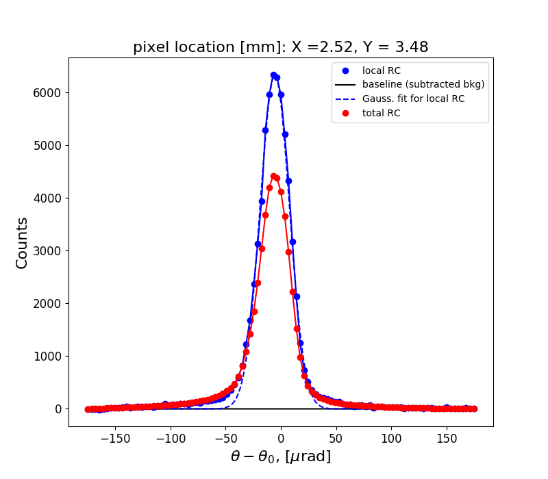
Figure 1 Rocking curves
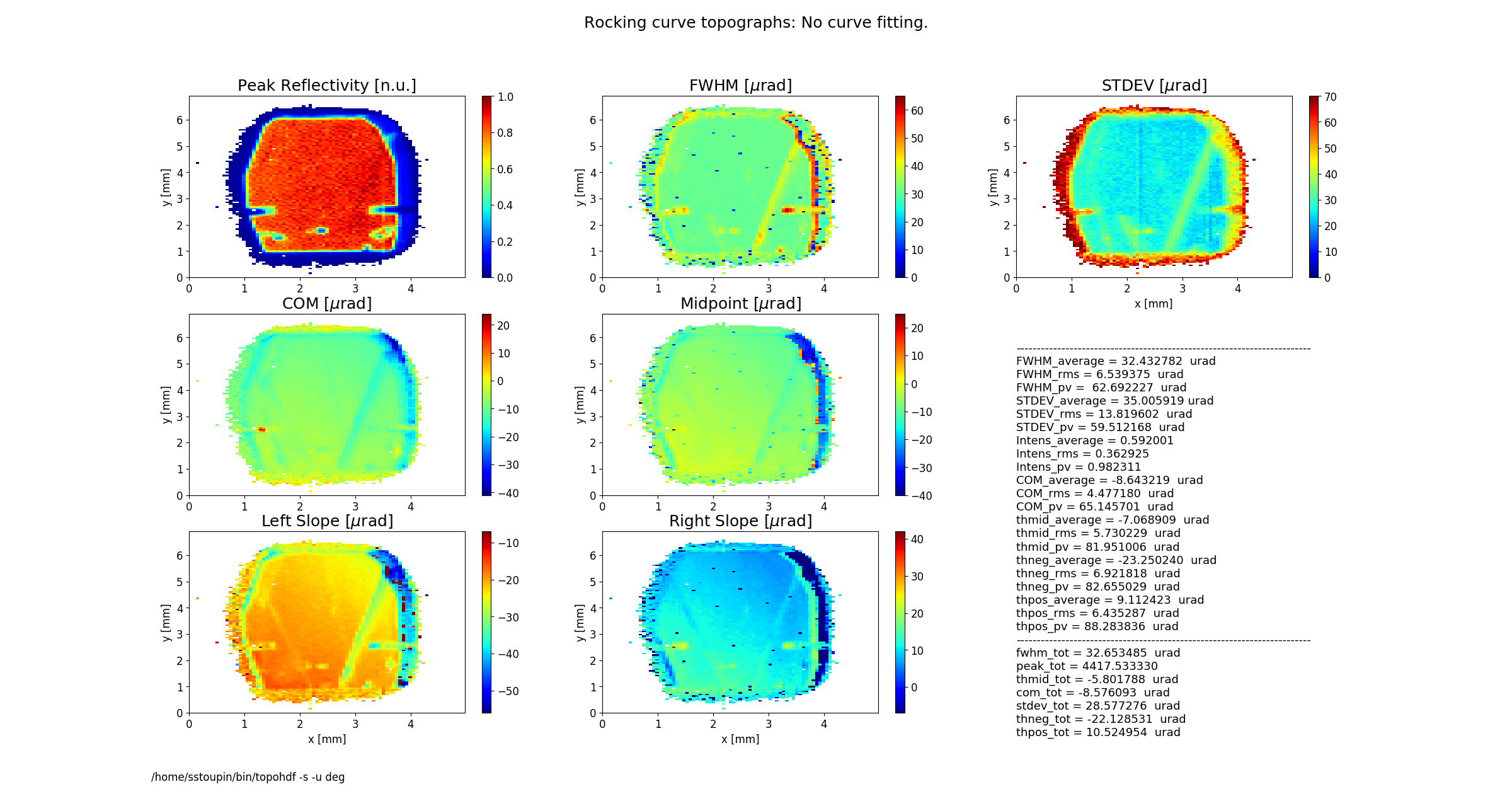
Figure 2 Rocking curve topographs
to better define crystal boundary (threshold for analysis), to obtain a smooth image (Gaussian fitting for each pixel), and to display the name of the sample in the figure title:
rctopo -t 1.1 -g -s -u deg -n diamond1 *hdf
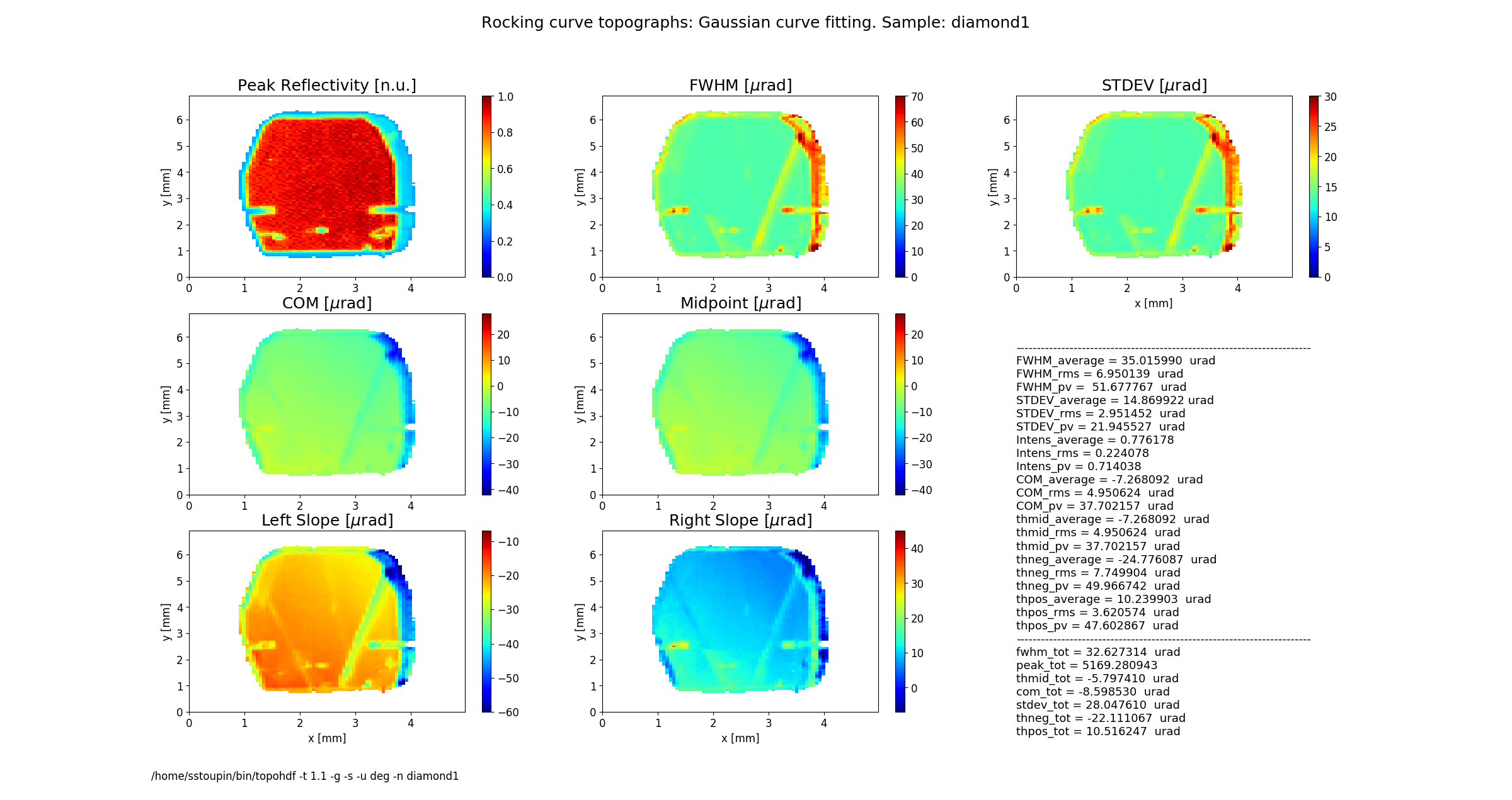
Figure 2 Rocking curve topographs
to select a region (the program assumes mm) and to perform statistical analysis and visualization over this region:
rctopo -r '1.5 3.5 4 6' -t 1.1 -g -s -u deg -n diamond1 *hdf
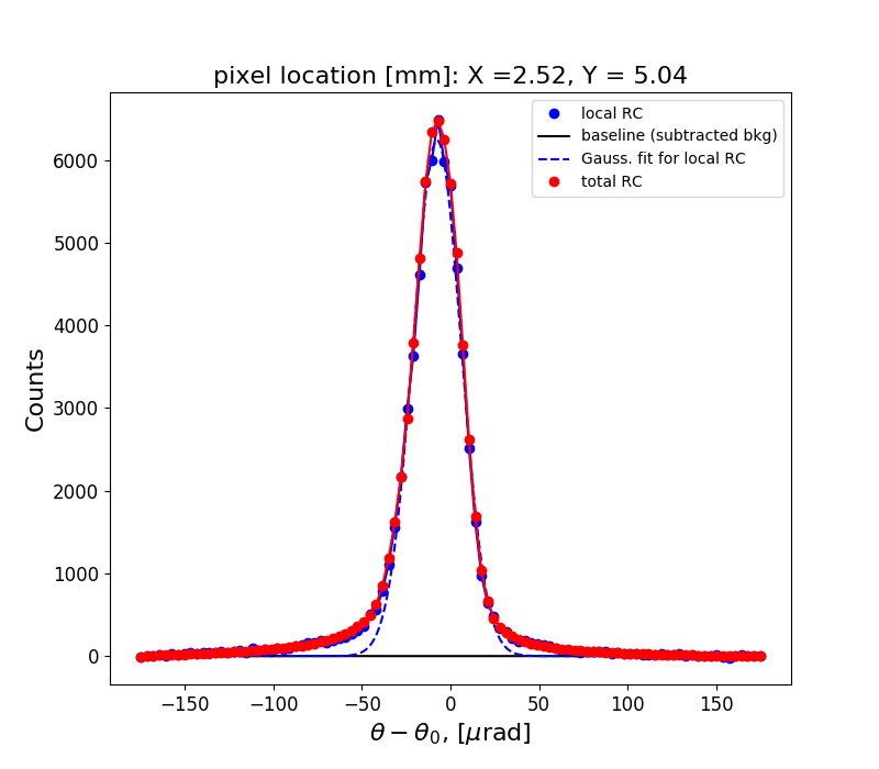
Figure 1 Rocking curves
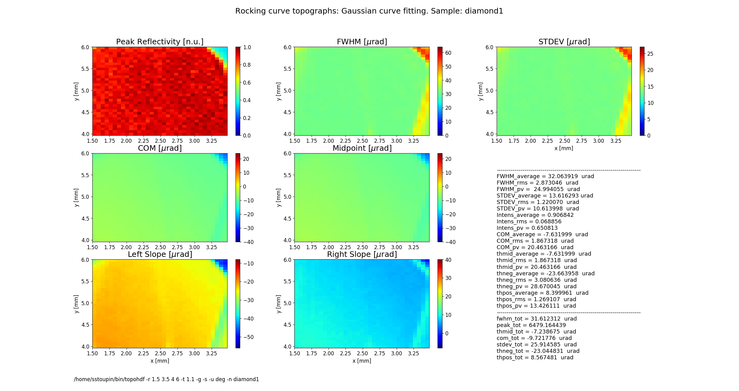
Figure 2 Rocking curve topographs
II. Rocking curve topography using HDF5 images and a configuration file ccd.py
The archive below contains a sequence of X-ray diffraction images embedded into h5 files (one file per image) of a diamond 111 crystal plate. The source was a bending magnet synchrotron beamline with a double-crystal Si (111) monochromator tuned to a photon energy of 8.05 keV. A strongly asymmetric Si (220) collimating (beam conditioning) crystal was used downstream the double-crystal monochromator. The original images collected using area detector PIXIS 1024F (pixel size of 13x13 um^2) were 4x4 binned to save space:
The input parameters are declated in the configuration file below. It should be placed in the working folder, which contains the archived .h5 images.
Note, that the configuration file includes paths within the .h5 file for the image array, theta and chi angles. Also, in this file no binning is declared rbin=1 because the original images are already binned 4x4. Otherwise, binning can be performed by the program (e.g., rbin=2 for 2x2 binning). Parameters tot_range and dyn_range define the upper limit of the dynamic range (these parameters are factors of the background level bkg0). The upper limit can be used to reject "hot" pixels.
To process the seqence of images using the instrument file (-i option):
rctopo -p -r '1 12.5 4.8 8.8' -t 10 -f 0.1 -m 0.1 -s -i -u urad C111*.h5
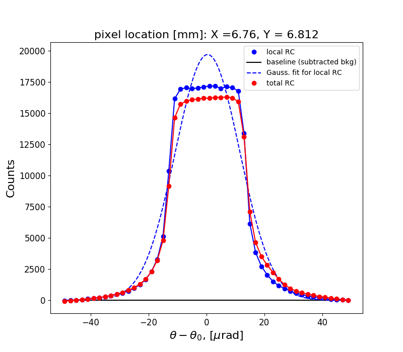
Figure 1 Rocking curves
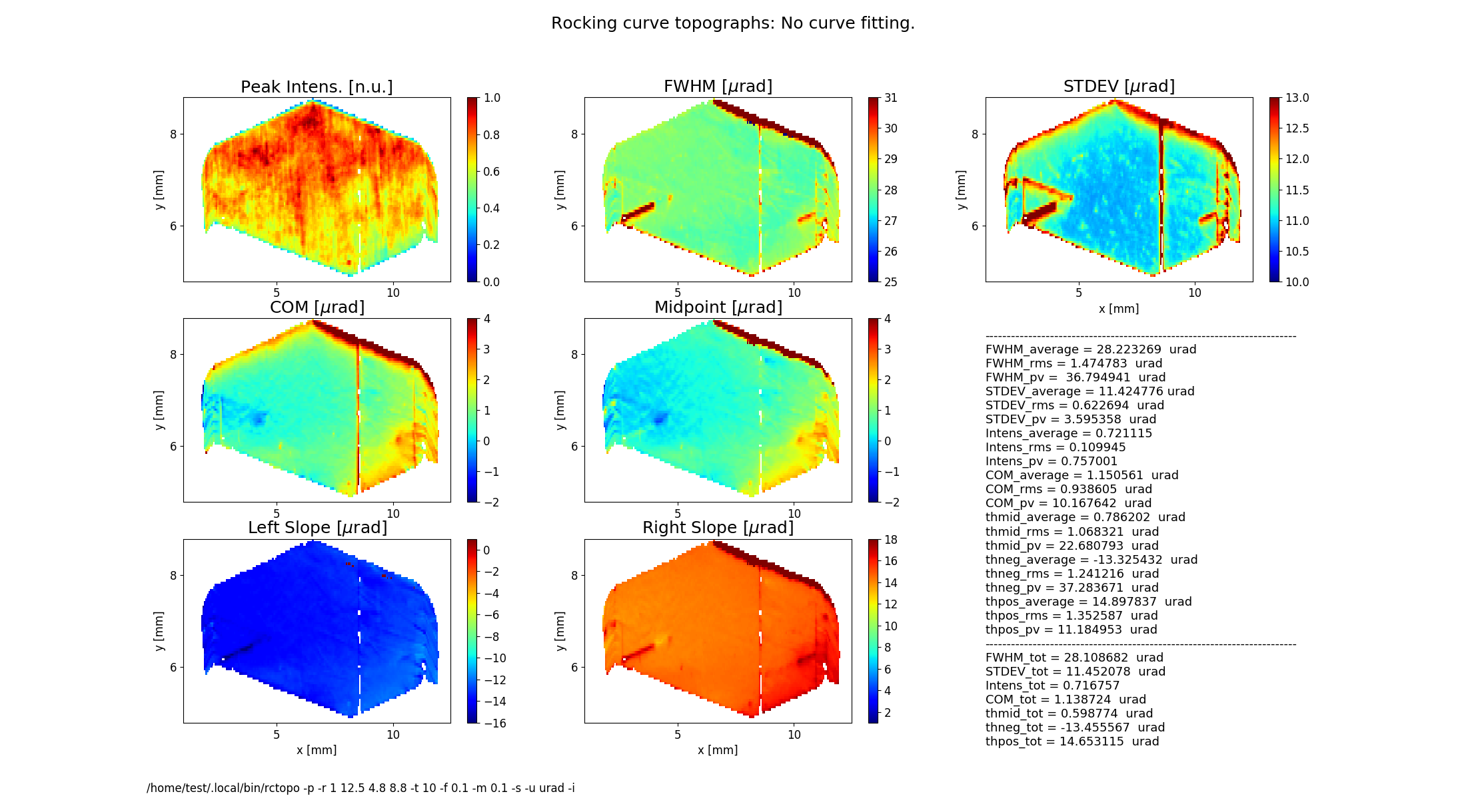
Figure 2 Rocking curve topographs
Here, option -p calls for a script (placed along with ccd.py in the current data folder):
An additional figure is generated having customized axes, titles, subplots, etc. This custom script (based on matplotlib commands and parameters) in principle can generate a publication-quality figure.
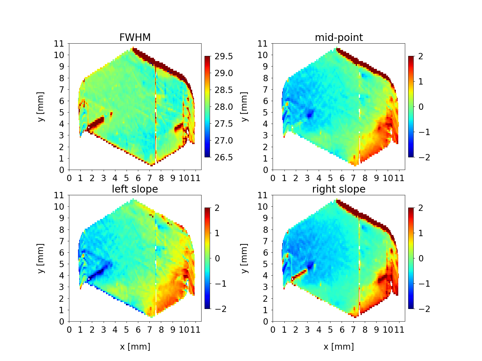
Figure 3 Rocking curve topographs (customized using figures.py)
The calculated topographs can be saved as data for post-processing/making custom figures. The results of calculations can be conveniently saved in one HDF5 metafile using --hdf option followed by a chosen filename:
rctopo --hdf5 topographs.hdf5 -r '1 12.5 4.8 8.8' -t 10 -f 0.1 -m 0.1 -s -i -u urad C111*.h5
The resulting metafile contains parameters of the calculation, topographs and curve statistics.
Below is an example of a script which reads the metafile, extracts the topographs and generates a figure in a format similar to the Figure 3 above.
Alternatively, the program can save individual topographs as images in .tif format (--tif option).
III. Analysis of transmission diffraction data
The archive of data below represents a sequence of transmission diffraction topographs of of a diamond (13 13 3) reflection in backscattering using a narrow bandwidth (1 meV) monochromatic x-rays. Instead of the Bragg angle of the crystal the photon energy of the incident x-ray beam (here in units of microradian) is scanned with small incremental steps.
The transmission diffraction data are processed using an option -c. In this mode the normal transmission level is subtracted from the data, the resulting difference is then inverted and treated as a reflectivity curve. In this mode the parameter bkg0 (from ccd.py) defines global threshold: data points with normal transmission baseline below bkg0 will be rejected.
The rejection threshold assigned through the option (-t 0.11 in this case) represents the least allowed fraction of the normal transmission level and should be always less than 1.0
rctopo -c -p -g -s -t 0.11 -r '0.2 1.3 0 1' -f 0.5 -m 0.5 -i -u urad *h5
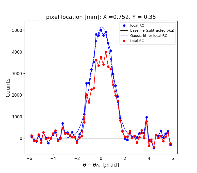
Figure 1 Inverted transmission diffraction curves
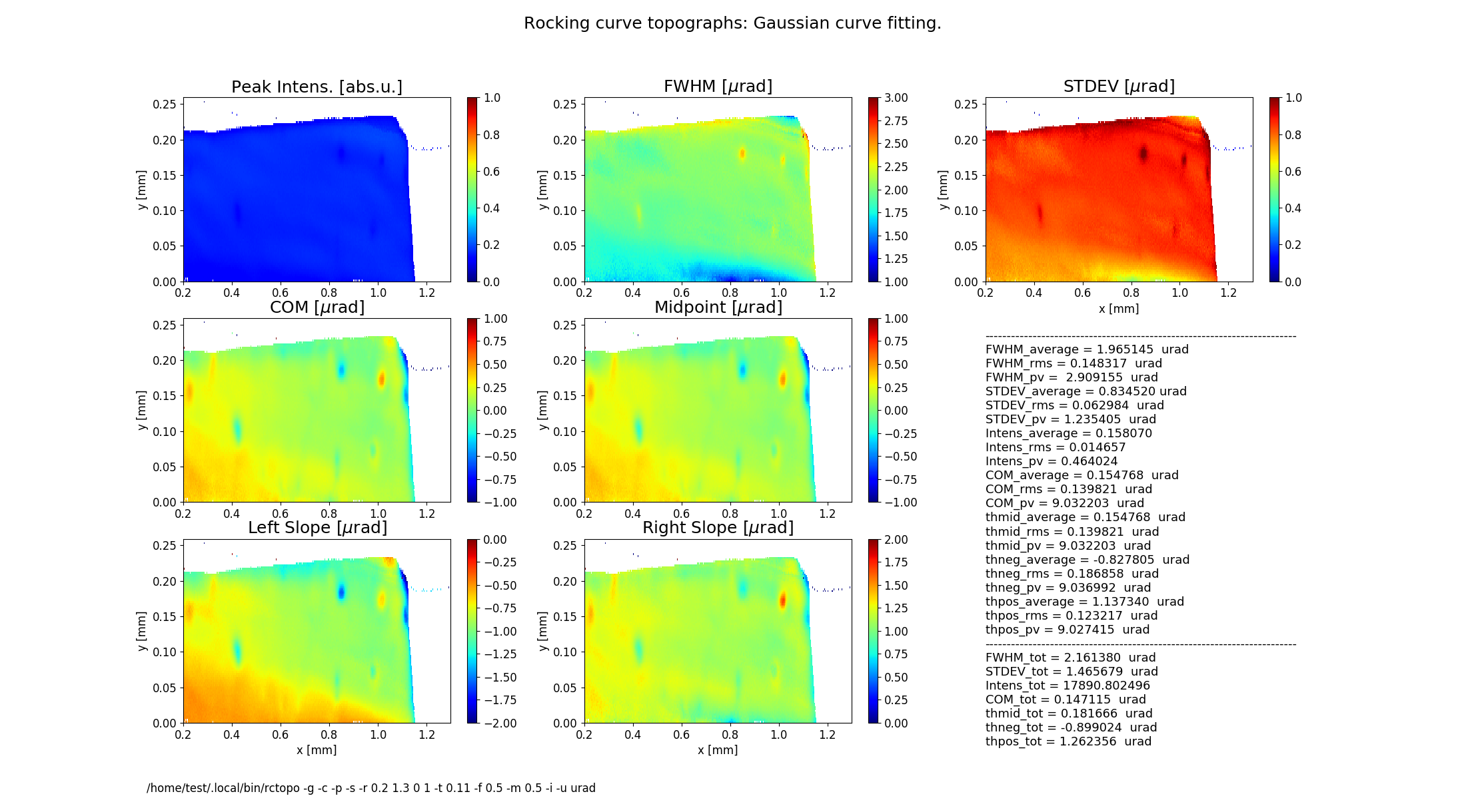
Figure 2 Inverted transmission diffraction topographs
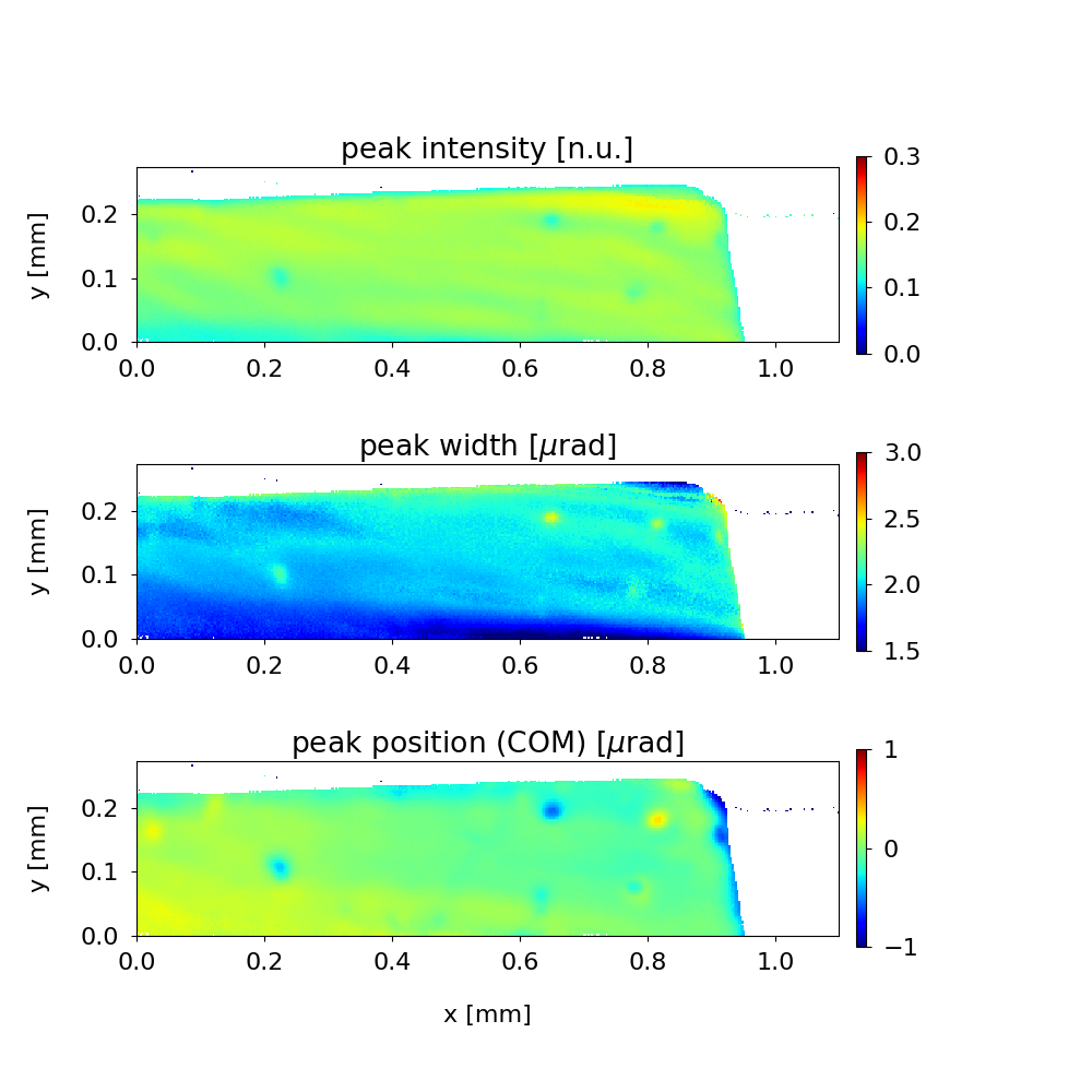
Figure 3 Inverted transmission diffraction topographs (customized using figures.py)
SEE ALSO
| author: | Stanislav Stoupin |
|---|---|
| email: | <sstoupin@gmail.com> |
| date: | Jun 12, 2020 |